Definition of diffusion models, a powerful new technique in artificial intelligence, involves gradually adding noise to an image and then reversing this process to generate a new image. This fascinating approach, explored through various types like DDPM and DDIM, has wide-ranging applications from image generation to restoration. Understanding the core concepts, mathematical foundations, and training processes behind these models is key to grasping their potential.
This exploration delves into the intricacies of diffusion models, providing a concise explanation of the fundamental steps, core concepts, and mathematical principles involved. From the probabilistic approach to the training process, we’ll uncover the nuances that make these models so revolutionary.
Introduction to Diffusion Models
Diffusion models are a revolutionary approach to generative tasks, particularly in image generation. They work by a clever process of gradually adding noise to an image and then reversing this process to create a new, original image. This seemingly simple concept has yielded impressive results, producing high-quality and diverse outputs. This approach differs significantly from traditional generative methods, offering a new paradigm for creating realistic synthetic data.The core idea behind diffusion models is to progressively corrupt a high-quality image with random noise, until it becomes indistinguishable from pure noise.
Then, the model learns to reverse this process, effectively denoising the image and reconstructing the original structure. This iterative denoising process, guided by the model’s learned parameters, allows it to generate entirely new, realistic images.
Diffusion Process Fundamentals
The diffusion process involves a series of steps where the input image is gradually transformed into noise. Each step involves adding a small amount of Gaussian noise to the previous image. Crucially, the model learns a mapping from the noisy images to the original clean image through this process. This mapping is captured in a series of carefully calculated steps.
Different Types of Diffusion Models
Various architectures exist for diffusion models, each with subtle variations in their implementation and performance. The key differences lie in how they reverse the diffusion process.
| Model Name | Core Concept | Key Characteristics |
|---|---|---|
| DDPM (Denoising Diffusion Probabilistic Models) | Learns a conditional probability distribution over the noise schedule. It employs a denoising network to progressively remove noise from noisy images. | Simpler architecture, relatively straightforward to implement. Can be computationally expensive for high-resolution images. |
| DDIM (Denoising Diffusion Implicit Models) | Provides a more efficient way to reverse the diffusion process by directly sampling from the denoising process. | Significantly faster than DDPM, allowing for faster generation of images. Might yield slightly lower quality in some cases compared to DDPM. |
| Improved DDPM variants (e.g., DDPM with variance scheduling, DDPM with adaptive noise schedule) | Address limitations of basic DDPM, enhancing the efficiency and quality of the diffusion process. | Focus on improving efficiency by optimizing the noise schedule and variance, often leading to improved image quality and faster training. |
These different models offer trade-offs between speed, quality, and computational resources. The choice of a specific model depends on the particular application and desired balance between these factors.
Mathematical Background
Diffusion models, at their core, are probabilistic frameworks. They leverage the power of stochastic processes to model the generation of data. Understanding the underlying mathematical principles is crucial for grasping the model’s inner workings and its remarkable ability to generate realistic data. This section delves into the core mathematical concepts and their practical application.
Probabilistic Approach
Diffusion models operate by gradually adding noise to an input data sample. This noise addition is meticulously controlled by a stochastic process. The crucial aspect is that this process is reversible. Crucially, the model learns to reverse this process, effectively denoising the data. This reversal is achieved through a carefully constructed probability distribution.
Diffusion Process Equations
The diffusion process itself is governed by a set of equations that dictate the evolution of the data as noise is added. A key equation is the transition probability: a probability of moving from one state (data point) to another (data point with added noise).
P(xt | x t-1)
This equation defines how the probability of observing a data point at a particular time step (t) depends on the data point at the previous time step (t-1). This relationship is crucial for understanding how the model learns to reverse the diffusion process.Another fundamental equation describes the noise schedule:
βt
This parameter controls the amount of noise added at each time step. A carefully designed schedule for β t is essential for effective denoising. The schedule is often a function of time t.
β1, β 2, …, β T
This sequence of values determines the amount of noise added in each step of the process.
Step-by-Step Demonstration
Imagine a data point x 0. The diffusion process begins by adding noise. The amount of noise added is determined by β 1. The new data point x 1 is calculated based on the previous data point and β 1. Then, in the next step, β 2 determines the amount of noise added to x 1 to obtain x 2.
This process repeats until x T is reached, which is a highly noisy version of x 0. The model learns to reverse this process by estimating the original data point x 0 from x T.
Diffusion models are fascinating, basically a way to generate realistic images by gradually adding noise and then reversing the process. While pondering these complex algorithms, I stumbled upon news about global reactions to Pope Francis’s passing. Lots of leaders and figures like JD Vance and even Donald Trump are offering tributes, as seen in this article pope francis death global leaders reactions tributes jd vance trump.
It’s interesting to consider how the human element intertwines with the technical innovations of diffusion models. Perhaps this interplay will lead to more meaningful and creative outputs in the future.
Role of Probability Distributions
Probability distributions are fundamental to diffusion models. The model learns a probability distribution, which captures the relationship between the noisy data points (x t) and the original data points (x 0). This is often a conditional distribution:
P(x0 | x T)
The goal is to approximate this distribution, which enables the model to sample from the original data distribution.
Comparison of Diffusion Models
| Model Type | Mathematical Foundation | Key Differences |
|---|---|---|
| Gaussian Diffusion | Uses Gaussian distributions to model the noise addition process. | Simpler to implement but might not be optimal for all data types. |
| Discrete Diffusion | Uses discrete steps to model the noise addition. | Often leads to better performance in some cases, particularly for image generation. |
| Non-Gaussian Diffusion | Employs non-Gaussian distributions to add noise, potentially capturing more complex relationships in data. | More complex to implement and potentially more computationally expensive. |
The table above presents a simplified comparison. Variations and nuances exist within each model type. The choice of model depends heavily on the specific application and the characteristics of the data being modeled.
Diffusion models, essentially, are algorithms that learn to reverse a process of adding noise to an image. This fascinating field is rapidly evolving, but it’s important to consider how these technologies might be misused, like the potential for negative influences in kid-targeted content, particularly on platforms like Netflix. The worrying trend of “kidfluencing” and its dark side, as discussed in this article about bad influence dark side of kidfluencing netflix , highlights the ethical considerations surrounding AI-generated content.
Ultimately, understanding diffusion models requires a nuanced perspective encompassing both their creative potential and the potential risks associated with their application.
Training Diffusion Models
Training diffusion models is a crucial step in leveraging their power for various tasks. The process involves meticulously guiding the model through a series of transformations, effectively teaching it to understand and generate intricate patterns within the training data. This process, though complex, is essential for unlocking the model’s potential to produce high-quality outputs.
Training Data Importance
The quality and quantity of the training data significantly impact the model’s performance. A diverse and representative dataset ensures the model grasps the nuances and variations within the subject matter. For example, a diffusion model trained on a limited dataset of images might struggle to generate images with uncommon characteristics. Conversely, a comprehensive dataset containing images from various angles, lighting conditions, and styles will result in a more robust and versatile model.
Objective Function and Optimization
The objective function guides the training process by defining the model’s goal. It quantifies how well the model is learning the distribution of the data. A common objective function used in diffusion models is minimizing the difference between the generated samples and the actual training data distribution. This minimization is typically achieved using optimization algorithms like stochastic gradient descent (SGD) or its variants.
These algorithms iteratively adjust the model’s parameters to improve its performance, gradually bringing the generated outputs closer to the target distribution.
Minimizing the difference between generated samples and the actual training data distribution is crucial for successful training.
Training Techniques
Several training techniques are employed to optimize diffusion models. These methods aim to enhance the model’s learning capabilities and stability. A critical technique is using techniques like data augmentation, which involves transforming the training data to create more varied and representative samples. This can improve the model’s generalization ability and robustness to different input variations.
- Data Augmentation: Transforming the training data (e.g., images) by applying rotations, flips, or color adjustments to increase the dataset’s size and variety. This aids in learning broader patterns and preventing overfitting to specific data characteristics.
- Learning Rate Scheduling: Adjusting the learning rate during training to prevent oscillations and ensure stable convergence to the optimal solution. This involves gradually decreasing the learning rate as training progresses, allowing the model to refine its parameters more precisely.
- Gradient Accumulation: Accumulating gradients over multiple mini-batches before updating the model’s parameters. This can be useful for handling large batches or datasets that don’t fit into memory at once, providing more stable updates to the model.
Fine-tuning on Specific Datasets
Fine-tuning a pre-trained diffusion model on a specific dataset allows adapting its capabilities to a particular task or domain. This process involves retraining the model on the new dataset, adjusting its parameters to better reflect the characteristics of the target data. For instance, a diffusion model trained on general images can be fine-tuned on medical images to improve its ability to generate or analyze such specialized imagery.
Training Flowchart
The training process involves a sequence of steps. This flowchart visualizes the process.
| Step | Description |
|---|---|
| 1. Data Preparation | Gathering and preprocessing the training data. This involves cleaning, formatting, and augmenting the data. |
| 2. Model Initialization | Creating a diffusion model with initial parameters. This often involves selecting an architecture and appropriate hyperparameters. |
| 3. Training Loop | Iteratively sampling data from the training set, running the diffusion process forward and backward, calculating the loss, and updating the model parameters. |
| 4. Evaluation | Assessing the model’s performance on a validation dataset to monitor progress and identify potential issues. |
| 5. Fine-tuning (Optional) | Adapting the model to a specific dataset or task. |
Applications of Diffusion Models: Definition Of Diffusion Models
Diffusion models, with their ability to generate realistic and diverse outputs, are rapidly transforming various fields. From creating stunning images to restoring damaged ones, these models are proving invaluable in AI. Their flexibility allows for applications beyond the realm of image processing, opening up exciting possibilities in fields like drug discovery and scientific research.The remarkable success of diffusion models stems from their unique approach to generating data.
By gradually adding noise to an image and then reversing the process, diffusion models learn the underlying patterns and distributions in the data. This allows them to produce outputs that are not just statistically plausible but often remarkably creative and evocative.
Diffusion models are essentially about gradually adding noise to an image, then learning to reverse that process and reconstruct the original. This concept, while seemingly abstract, is now finding practical applications in various fields. Considering recent events like China imposing tariffs on imports of all US products, this trade war might lead to a surge in demand for domestic AI solutions, further driving innovation in diffusion models and their associated technologies.
It’s an interesting interplay of global economics and cutting-edge tech. Ultimately, the potential of diffusion models remains vast.
Image Generation
Diffusion models have revolutionized image generation, surpassing previous methods in terms of realism and detail. They can generate high-resolution images of diverse subjects, from intricate landscapes to detailed portraits, often exceeding the capabilities of generative adversarial networks (GANs). These models learn the complex relationships between image features, enabling them to create novel and compelling imagery. For example, a diffusion model can be trained on a dataset of photographs of cats and then generate new images of cats with varying fur patterns and poses.
This ability has significant implications in art, design, and entertainment.
Image Restoration
Diffusion models are not just for generating new images; they are also adept at restoring damaged or degraded ones. By reversing the noise addition process, they can effectively fill in missing details and reduce artifacts, enhancing the quality of images that have been corrupted by noise, blur, or other imperfections. This application has practical value in fields like archaeology, where faded or damaged historical images can be restored to a higher quality.
Imagine an ancient painting damaged by time, which can be restored with diffusion models, revealing details lost to the passage of centuries.
Other Applications
Beyond image generation and restoration, diffusion models have applications across diverse domains. They are being used to generate 3D models, create realistic audio, and even synthesize music. Their potential extends to drug discovery, where they can generate molecules with specific properties, and scientific research, where they can generate realistic simulations. Their flexibility allows them to be adapted to a wide range of tasks, making them a powerful tool in the AI arsenal.
Table of Use Cases
The following table highlights some specific use cases of diffusion models in various domains.
| Domain | Specific Use Case |
|---|---|
| Image Generation | Creating photorealistic images of diverse subjects, generating artistic styles |
| Image Restoration | Restoring damaged or degraded images, enhancing image quality |
| 3D Modeling | Generating 3D models from 2D images or sketches |
| Audio Synthesis | Creating realistic audio, including speech and music |
| Drug Discovery | Generating molecules with specific properties, accelerating drug development |
Potential Future Applications
The potential of diffusion models extends far beyond current applications. Their adaptability and ability to learn complex distributions suggest exciting future applications in fields like personalized medicine, where they could generate personalized treatment plans, or in scientific research, where they could simulate complex phenomena with unprecedented realism. Researchers are actively exploring their use in creating more sophisticated and intelligent AI agents.
Advantages and Disadvantages

Diffusion models have revolutionized image generation, offering impressive results. However, like any powerful technology, they come with their own set of trade-offs. Understanding these strengths and weaknesses is crucial for effectively leveraging their potential and mitigating their limitations. This section will delve into the advantages and disadvantages of diffusion models, comparing them to other methods and analyzing their computational demands.
Strengths of Diffusion Models, Definition of diffusion models
Diffusion models excel at generating high-quality, diverse images. Their ability to capture complex relationships and intricate details in generated content is a significant advantage. This is often achieved through iterative refinement of the latent space, leading to superior results compared to previous methods. They often surpass GANs in terms of qualitative image quality. Another strength lies in their versatility.
They can be adapted for various tasks beyond image generation, including inpainting, super-resolution, and style transfer.
Weaknesses of Diffusion Models
Despite their strengths, diffusion models are not without limitations. Training diffusion models requires substantial computational resources, including high-performance GPUs and vast datasets. This makes them inaccessible to many researchers and practitioners with limited computational infrastructure. The training process itself can be time-consuming, requiring significant resources and expertise. Furthermore, the generation process can also be computationally expensive, leading to longer inference times compared to some alternative models.
The inherent iterative nature of diffusion models adds to the computational burden, making it a critical consideration.
Comparison to Other Image Generation Methods
Diffusion models are often compared to Generative Adversarial Networks (GANs). GANs, while capable of producing impressive results, often suffer from issues like mode collapse (generating images that cluster around a few similar samples) and instability during training. Diffusion models, on the other hand, are generally more stable and capable of generating a wider variety of outputs. Variational Autoencoders (VAEs) can also be used for image generation, but they typically produce less visually appealing results and struggle with capturing intricate details found in high-quality images.
In summary, diffusion models offer a more robust and reliable approach to image generation compared to GANs and VAEs.
Computational Requirements
Training and using diffusion models requires significant computational resources. The sheer size of the datasets and the complex nature of the models necessitate high-performance GPUs and significant memory. The iterative nature of the training process further exacerbates the computational demand. Inference, or generating new images, also demands considerable computational power, potentially affecting the speed and practicality of use cases.
Limitations and Areas for Improvement
Diffusion models have limitations that researchers are actively addressing. The high computational cost remains a significant barrier to wider adoption. Furthermore, the generation process can be slow. Researchers are exploring ways to reduce these computational burdens, potentially through optimizing the model architecture or developing more efficient sampling techniques. Addressing these challenges will be key to democratizing access to these powerful image generation tools.
Further research also focuses on improving the diversity and quality of generated images, and addressing potential biases in the training data.
Summary Table
| Feature | Advantages | Disadvantages |
|---|---|---|
| Image Quality | High-quality, diverse images; often surpassing GANs | Potential for slow generation, especially for complex scenes |
| Versatility | Adaptable for various tasks beyond image generation (e.g., inpainting, super-resolution) | Requires substantial computational resources for training |
| Stability | Generally more stable during training than GANs | Computational cost for inference is high |
| Computational Cost | Can capture complex relationships and details | Training time can be extensive |
| Comparison to other methods | Generally more robust and reliable compared to GANs and VAEs | Potential for bias in generated images if training data is biased |
Image Generation with Diffusion Models
Diffusion models excel at generating realistic images, a capability that stems from their unique training approach. Instead of directly learning image representations, they progressively add noise to an image, then reverse this process to reconstruct it. This probabilistic approach allows for the creation of novel images, as the model learns the underlying distribution of image data. This process is computationally intensive but yields visually compelling results.The core idea behind image generation with diffusion models is to learn the reverse process of how an image is corrupted by noise.
By training on a vast dataset of images, the model can effectively learn the intricate relationships and patterns within the data. This learned knowledge is then leveraged to generate new, unseen images that resemble the training data in style and content.
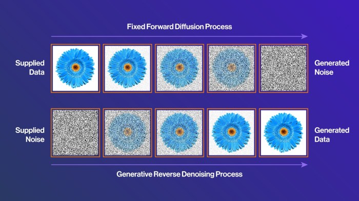
Image Generation Process
Diffusion models operate by gradually adding noise to an input image until it becomes a random noise vector. This process, called forward diffusion, can be visualized as a series of steps where the image is progressively transformed into pure noise. The model learns to predict the noise added in each step. The reverse process, called reverse diffusion, aims to reconstruct the original image from the pure noise by gradually removing the noise.
The model’s training focuses on predicting the noise at each step of the reverse process, thereby learning the underlying distribution of the training data.
Reverse Diffusion Steps
The reverse diffusion process involves a series of steps, each designed to remove a portion of the added noise. Each step involves a denoising process, where the model predicts the noise added at that step and subtracts it from the noisy image. The model is trained to predict the noise in each step from the noisy image. This iterative process is repeated until the model produces a nearly noise-free image.
Controlling Generated Image Characteristics
Various techniques allow for controlling the characteristics of the generated images. One approach involves using conditional diffusion models, where the model is conditioned on specific text prompts. This allows for generating images that match the specified text description. Another approach involves using latent space manipulation. By altering the latent representation of the image, you can influence its style or content.
Fine-tuning for Specific Styles
Fine-tuning a diffusion model for specific styles involves training the model on a dataset of images with the desired style. This allows the model to learn the unique characteristics of that style, enabling it to generate images that closely resemble it. For instance, if the goal is to generate images in the style of Van Gogh, the model would be trained on a dataset of Van Gogh’s paintings.
The model will learn the specific brushstrokes, color palettes, and composition techniques associated with Van Gogh’s style.
Workflow Diagram
+-----------------+        +-----------------+
|  Input Image    |------>|  Forward Diffusion |
+-----------------+        +-----------------+
|      |             |      |   Adding Noise    |
|      |             |      |   Iteratively    |
|      v             |      |                   |
+-----------------+        +-----------------+
| Noisy Image      |------>|  Reverse Diffusion  |
+-----------------+        +-----------------+
|      |             |      |   Removing Noise   |
|      |             |      |   Iteratively    |
|      v             |      |                   |
+-----------------+        +-----------------+
| Generated Image  |--------|                   |
+-----------------+        +-----------------+
Image Restoration and Enhancement
Diffusion models offer powerful capabilities for image restoration and enhancement, going beyond simple noise reduction.
They can effectively address various image degradation issues, such as blurring, compression artifacts, and damage, by learning the underlying data distribution. This ability to model complex transformations allows for more sophisticated and accurate restorations compared to traditional methods. The inherent probabilistic nature of diffusion models enables them to fill in missing information or details while preserving the original image’s content.
Image Restoration Techniques with Diffusion Models
Diffusion models excel at image restoration tasks by learning the underlying distribution of clean images. They can effectively reverse the degradation process, learning the inverse mapping from corrupted images to their original counterparts. This is achieved through a training process that involves gradually adding noise to clean images and then learning to reverse this process. By learning the noise-removal process, the model can restore images that have been subjected to various degradations.
This capability is particularly valuable in scenarios involving noisy or damaged images, where the goal is to recover the original, pristine image.
Enhancement Techniques Using Diffusion Models
Diffusion models can also enhance images by increasing their resolution or improving their visual quality. This is done by leveraging the learned probabilistic model to generate higher-resolution versions of the input image. By iteratively refining the image based on the learned distribution, the model can add details and sharpen features, improving the overall visual appeal. This process is akin to super-resolution, but with the advantage of preserving the overall content and style of the original image.
Furthermore, they can adjust image contrast, color balance, and other visual aspects to produce a desired output.
Examples of Image Restoration and Enhancement
One example of image restoration is the recovery of a blurry image. A diffusion model can analyze the blurry image and reconstruct a sharper version by learning the relationship between the blurry and clear image representations. Another example is restoring an image with significant damage or missing parts. The model can analyze the existing parts of the image and fill in the missing regions while maintaining the image’s overall structure and content.
Examples of enhancement include increasing the resolution of a low-resolution image, enhancing the clarity of an image with poor lighting, or removing noise from a photograph.
Comparison of Methods
Traditional image restoration methods often rely on specific algorithms for specific types of degradation. Diffusion models, however, offer a more general approach by learning a probabilistic model that encompasses various degradation types. This makes them adaptable to a wider range of restoration and enhancement tasks. However, the training process for diffusion models can be computationally expensive and require large datasets.
Table: Image Restoration Tasks and Diffusion Model Solutions
| Image Restoration Task | Diffusion Model Solution |
|---|---|
| Removing noise from an image | The model learns the noise distribution and reverses the process to remove noise from the image. |
| Restoring a blurry image | The model learns the relationship between blurry and clear images and reconstructs a sharper version. |
| Repairing damaged or missing parts of an image | The model learns from existing parts and fills in the missing regions while maintaining the overall structure and content. |
| Increasing image resolution | The model generates a higher-resolution version of the image, adding details and sharpening features while preserving the original content. |
Evaluation Metrics
Diffusion models, while powerful, require rigorous evaluation to assess their performance accurately. Different metrics are employed depending on the specific application, ranging from image generation to inpainting. A crucial aspect of evaluating these models is understanding their strengths and weaknesses in various tasks. This section delves into the diverse metrics used to evaluate diffusion models, their rationale, limitations, and practical application with illustrative examples.
Quantitative Metrics for Image Quality
Understanding how well a diffusion model generates images requires objective measurements. Quantitative metrics assess image quality by comparing generated images to ground truth or reference images. These metrics are essential for objectively comparing different diffusion models and evaluating their performance.
- Peak Signal-to-Noise Ratio (PSNR): PSNR quantifies the difference between the generated image and the ground truth image by measuring the ratio of the maximum possible power of a signal to the power of corrupting noise. Higher PSNR values indicate a better match between the generated image and the ground truth image, signifying better image quality. The formula for PSNR is: PSNR = 10
– log 10(MAX 2/MSE), where MAX is the maximum pixel value (typically 255 for 8-bit images) and MSE is the mean squared error. - Structural Similarity Index (SSIM): SSIM measures the structural similarity between two images, considering luminance, contrast, and structure. It provides a more comprehensive assessment of image quality than PSNR, as it accounts for perceived visual differences. Higher SSIM values indicate greater structural similarity, implying better image quality.
- Multi-Scale Structural Similarity Index (MS-SSIM): MS-SSIM extends the SSIM metric by considering the image structure at different scales. This is particularly useful for evaluating images with complex textures or details. This enhanced approach provides a more robust measure of structural similarity across various resolutions and image characteristics.
Qualitative Metrics and User Studies
Qualitative metrics are crucial for understanding the subjective aspects of image quality, which are not fully captured by quantitative metrics. User studies are often conducted to evaluate the perceptual quality of generated images.
- Human Evaluation: Human judgment plays a critical role in assessing the visual quality of generated images. Expert evaluators or representative user groups can rate images based on various criteria, including realism, detail, and aesthetic appeal. This approach provides valuable insight into the subjective preferences and perceptions related to image quality.
- Inpainting Quality Assessment: For tasks like inpainting, the evaluation metrics need to consider the fidelity of the inpainted region, smoothness, and the preservation of the surrounding image content. Metrics tailored to these specific aspects of inpainting are often necessary to provide a complete assessment.
Table of Evaluation Metrics
| Metric | Description | Strengths | Limitations |
|---|---|---|---|
| PSNR | Peak Signal-to-Noise Ratio | Simple to calculate, widely used | Doesn’t capture perceptual quality, sensitive to outliers |
| SSIM | Structural Similarity Index | Considers structural similarity, more perceptually relevant | Computationally more expensive than PSNR |
| MS-SSIM | Multi-Scale Structural Similarity Index | Captures structural similarity at multiple scales | Computationally more expensive than SSIM |
| Human Evaluation | Expert or user judgments | Captures subjective preferences, comprehensive | Time-consuming, prone to bias |
Example Calculation (PSNR)
Suppose a ground truth image and a generated image have the following mean squared error (MSE): MSE =
100. The maximum pixel value is MAX =
255. Then, the PSNR is calculated as: PSNR = 10
– log 10(255 2/100) ≈ 28.4 dB.
Ending Remarks
In conclusion, diffusion models offer a compelling blend of theoretical depth and practical application, revolutionizing image generation and restoration. Their ability to learn from data and generate novel outputs makes them a fascinating field of study. While computational resources are a factor, the potential advantages and future applications of these models are vast, promising exciting developments in the realm of artificial intelligence.